This repository is for the data and code presented in the paper published here (to be added).
Install packages
Firstly, you will need to install the VarReg package and
a few others to perform the code below.
CD4 dataset
This dataset is located within the gamlss package. CD4
is a type of white blood cell, and in this dataset, it has been measured
in uninfected children born from HIV-1 infected women. The dataset
contains 609 measurements of CD4 cell counts and the child’s age at
which the measurements were taken.
data("CD4")

str(CD4)
#> 'data.frame':    609 obs. of  2 variables:
#>  $ cd4: num  387 2183 904 1681 656 ...
#>  $ age: num  4.5 0.83 2.06 1.44 2.67 1.17 1.94 1.72 2.54 1.66 ...
Lets reproduce the graphic in the paper, showing that at younger ages there is more variation in the CD4 counts than at older ages, demonstrating heteroscedasticity.
ggplot(data=CD4, aes(y=cd4, x=age)) +
  geom_point()+
  xlab("Age of child in years")+
  ylab("CD4 cell count")+
  theme_minimal()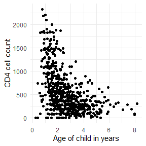
CD4 dataset: more variation in the CD4 counts at younger ages than at older ages
Linear model in mean and variance
Let us fit a linear model in the mean and variance model, like so
cd4.linear<-semiVarReg(y = CD4$cd4,
                       x=CD4$age,
                       meanmodel = "linear",
                       varmodel = "linear",
                       maxit=10000)
key outputs for model fit:
cd4.linear$aic
#> [1] 8999.12
cd4.linear$bic
#> [1] 9016.767
Key estimates from model:
cd4.linear$mean
#> Intercept   CD4$age
#>  884.7263 -124.8084
cd4.linear$variance
#> Intercept   CD4$age
#> 218069.56 -23922.79
Visualise the model with plotVarReg function:
plotVarReg(cd4.linear, xlab = "Age in years", ylab = "CD4 cell count")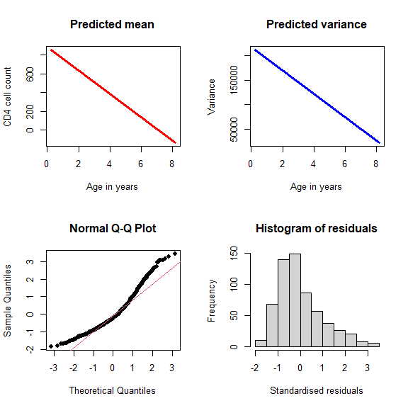
PlotVarReg example
Searching for the optimal spline
Searching to a max of 7 knots in the mean and variance, with maximum
iterations (maxit) of 100 to minimise time taken for the
search:
cd4.best <- searchVarReg(y=CD4$cd4,
                         x=CD4$age,
                         maxknots.m = 7,
                         maxknots.v = 7,
                         selection="AIC",
                         maxit=100)
lets look at the AIC table to identify where the best model is located:
cd4.best$AIC %>%
kbl(digits=1)| Mean_zero | Mean_constant | Mean_linear | Mean_Knot0 | Mean_Knot1 | Mean_Knot2 | Mean_Knot3 | Mean_Knot4 | Mean_Knot5 | Mean_Knot6 | Mean_Knot7 | |
|---|---|---|---|---|---|---|---|---|---|---|---|
| Var_constant | 9750.8 | 9205.7 | 9044.1 | 8995.6 | 8997.3 | 8977.0 | 8972.1 | 8967.6 | 8966.3 | 8964.8 | 8964.6 |
| Var_linear | 9662.4 | 9157.1 | 8999.8 | 8919.5 | 8916.2 | 8893.4 | 8889.8 | 8886.4 | 8885.6 | 8884.5 | 8884.7 |
| Var_Knot0 | 9554.9 | 9157.1 | 8947.8 | 8839.2 | 8834.9 | 8862.5 | 8890.6 | 8905.7 | 8912.8 | 8916.5 | 8920.8 |
| Var_Knot1 | 9569.4 | 9071.5 | 8904.2 | 8843.9 | 8843.7 | 8827.6 | 8825.4 | 8823.6 | 8823.3 | 8822.8 | 8823.6 |
| Var_Knot2 | 9529.3 | 8998.8 | 8897.0 | 8842.4 | 8843.9 | 8810.5 | 8804.0 | 8799.1 | 8797.8 | 8797.3 | 8798.5 |
| Var_Knot3 | 9524.5 | 8989.1 | 8892.3 | 8845.5 | 8847.5 | 8809.0 | 8802.2 | 8797.2 | 8796.2 | 8795.6 | 8796.8 |
| Var_Knot4 | 9526.0 | 8989.6 | 8893.1 | 8848.0 | 8849.8 | 8813.2 | 8805.8 | 8801.3 | 8800.6 | 8800.2 | 8801.3 |
| Var_Knot5 | 9525.9 | 8985.4 | 8894.0 | 8849.5 | 8851.4 | 8809.1 | 8803.7 | 8800.0 | 8799.1 | 8798.9 | 8800.1 |
| Var_Knot6 | 9527.4 | 8987.0 | 8895.1 | 8851.7 | 8853.6 | 8810.9 | 8804.9 | 8801.3 | 8800.6 | 8800.4 | 8801.4 |
| Var_Knot7 | 9530.4 | 8988.6 | 8896.6 | 8852.4 | 8854.2 | 8813.2 | 8807.9 | 8804.3 | 8803.4 | 8803.2 | 8804.4 |
The best model is saved within the cd4.best list. The
key estimates from the best model are:
cd4.best$best.model$knots.m
#> [1] 6
cd4.best$best.model$knots.v
#> [1] 3

cd4.best$best.model$mean
#>    Intercept M_Knt6_Base1 M_Knt6_Base2 M_Knt6_Base3 M_Knt6_Base4 M_Knt6_Base5 M_Knt6_Base6 M_Knt6_Base7
#>     32.98833   1597.06078    713.32197    582.58478    472.08281    291.50092    269.24506    220.66235
#> M_Knt6_Base8
#>    155.83254
cd4.best$best.model$variance
#>    Intercept V_Knt3_Base1 V_Knt3_Base2 V_Knt3_Base3 V_Knt3_Base4 V_Knt3_Base5
#>   40801.4581  411830.6370  109290.5901    2784.9777     914.4245  -25616.3670
ie. 6 knots in mean and 3 in variance, with parameter estimates as given. We can then plot this best model:
plotVarReg(cd4.best$best.model,
           xlab = "Age in years",
           ylab = "CD4 cell count")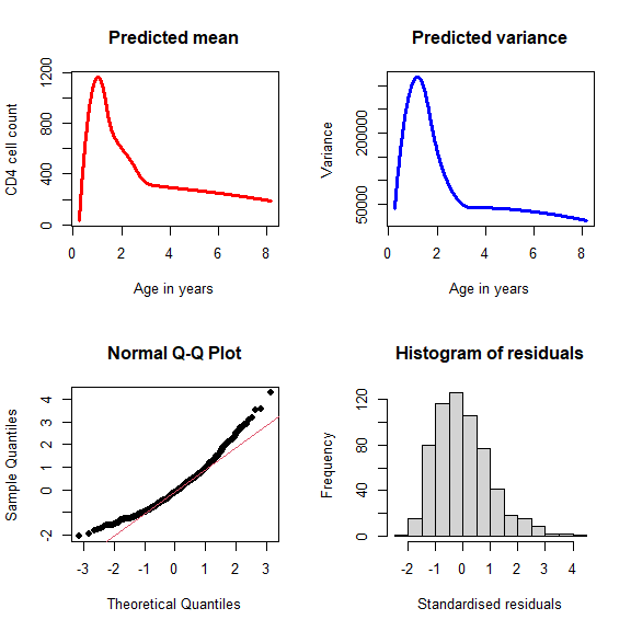
plotVarReg example of best model from search VarReg
From these residuals, there still appears to be deviations from normality in the residuals, again seen in both the Q-Q plot and the histogram. Therefore the incorporation of a shape parameter should be investigated.
lssVarReg function
In order to fit models with a shape parameter, we utilise the
lssVarReg() function. Firstly, let us fit a constant shape
parameter with 6 knots in the mean and 3 knots in the variance, that
is,
Let us fit two models, one with a constant shape parameter and one with a linear model in the shape, with the following code.
con.shape<-lssVarReg(y=CD4$cd4,
                     x=CD4$age,
                     locationmodel="semi",
                     knots.l=6,
                     scale2model="semi",
                     knots.sc=3,
                     mono.scale = "inc",
                     shapemodel="constant",
                     maxit=1000 )

linear.shape<-lssVarReg(y=CD4$cd4,
                        x=CD4$age,
                        locationmodel="semi",
                        knots.l=6,
                        scale2model="semi",
                        knots.sc=3,
                        shapemodel="linear",
                        int.maxit=1000,
                        print.it=TRUE,
                        maxit=1000 )
If we want to speed up the model, we can use starting estimates (from our best model) and parameter space restrictions, like so for the constant model:
con.shape_faster <- lssVarReg(y=CD4$cd4, x=CD4$age,
                              locationmodel="semi",
                              knots.l=6,
                              scale2model="semi",
                              knots.sc=3,
                              shapemodel="constant",
                              para.space="positive",
                              location.init = cd4.best$best.model$mean,
                              scale2.init = cd4.best$best.model$variance,
                              int.maxit = 10000,
                              maxit=1000 )
And compare the models as we did in the paper:
data.frame(Model = c("No shape", "Constant shape", "Linear shape"),
           AIC = c(cd4.best$best.model$aic, con.shape$aic, linear.shape$aic),
           BIC = c(cd4.best$best.model$bic, con.shape$bic, linear.shape$bic)) %>%
  kbl(digits=1,
      align='c',
      caption = "Comparison of AIC from shape models for CD4 cell counts.") %>%
kable_paper(full_width = TRUE )| Model | AIC | BIC |
|---|---|---|
| No shape | 8795.6 | 8861.8 |
| Constant shape | 8697.7 | 8768.3 |
| Linear shape | 8687.1 | 8762.1 |
And compare the residuals:
n<-length(CD4$age)
knot6<-bs(CD4$age, df= 8, degree=2)
knot3<-bs(CD4$age, df= 5, degree=2)

##normal model
npred.mean<-colSums(t(cbind(rep(1,n),knot6))*cd4.best$best.model$mean)
npred.var<-colSums(t(cbind(rep(1,n),knot3))*cd4.best$best.model$variance)

stand.res<- (CD4$cd4-npred.mean)**2/(npred.var)
chiq<-qchisq(c(1:n)/(n+1), df=1)

#constant residuals
con.res<-lss_calc(con.shape)
con.res<-con.res[order(con.res$CD4.age),]

#linear residuals
lin.res<-lss_calc(linear.shape)
lin.res<-lin.res[order(lin.res$CD4.age),]

par(mfrow=c(1,3))
plot(chiq, sort(stand.res), main=NULL, ylim=c(0, 10), pch=19, ylab="Squared standardised residuals after fit with no shape", xlab="Chi-Square(1) quantiles")
abline(0,1)
mtext('A', side=3, line=2, at=0, adj=3)

plot(chiq, sort(con.res$stand.res2), main=NULL, ylim=c(0, 10),pch=19, ylab="Squared standardised residuals after LSS (constant) fit", xlab="Chi-Square(1) quantiles")
abline(0,1)
mtext('B', side=3, line=2, at=0, adj=3)
plot(chiq, sort(lin.res$stand.res2), main=NULL, ylim=c(0, 10),pch=19, ylab="Squared standardised residuals after LSS (linear) fit", xlab="Chi-Square(1) quantiles")
abline(0,1)
mtext('C', side=3, line=2, at=0, adj=3)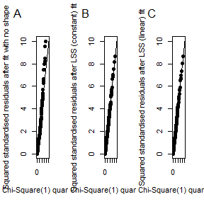
Comparison of residuals
Viral load dataset (censored outcome data)
This is a dataset of the HIV viral load (blood concentration of HIV RNA on a log10 scale) measured in 257 participants. Prior to commencing a clinical trial, participants had their blood assayed twice during a short period of time. Although the underlying viral load is unchanged in this time, the readings will differ due to measurement error. Another important aspect is that measurements cannot be detected below a particular assay limit, in this case, 2.70.
Lets plot the data:
ggplot(rna, aes(x=x, y=y))+
  geom_point()+
  geom_hline(yintercept = 0)+
  xlab("Mean viral load")+
  ylab("Difference in viral load")+
  theme_minimal()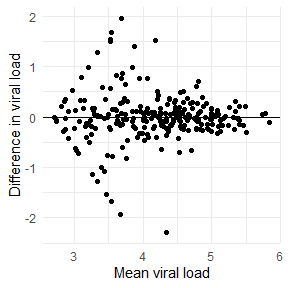
Viral load data demonstrating measurement error
Now let us search for the optimal knots, using the censoring indicator and
Monotonic decreasing model:
rna.best <- searchVarReg(y=rna$y,
                         x=rna$x,
                         maxknots.m = 5,
                         maxknots.v = 5,
                         mono.var = "dec",
                         selection="AIC",
                         maxit=1000)
AIC from all models:
rna.best$AIC %>%
kbl(digits=1)| Mean_zero | Mean_constant | Mean_linear | Mean_Knot0 | Mean_Knot1 | Mean_Knot2 | Mean_Knot3 | Mean_Knot4 | Mean_Knot5 | |
|---|---|---|---|---|---|---|---|---|---|
| Var_constant | 356.6 | 358.6 | 360.7 | 362.4 | 364.4 | 366.8 | 367.6 | 368.0 | 370.2 |
| Var_linear | 343.7 | 345.0 | 346.6 | 343.8 | 346.0 | 346.8 | 348.2 | 349.7 | 351.9 |
| Var_Knot0 | 308.8 | 310.4 | 312.4 | 314.0 | 314.7 | 316.5 | 318.5 | 319.1 | 321.2 |
| Var_Knot1 | 301.4 | 303.1 | 305.0 | 306.8 | 307.9 | 309.2 | 311.5 | 311.8 | 313.6 |
| Var_Knot2 | 300.2 | 301.7 | 303.7 | 305.3 | 306.4 | 308.0 | 310.2 | 310.3 | 312.2 |
| Var_Knot3 | 300.9 | 302.6 | 304.5 | 306.0 | 307.2 | 308.8 | 310.9 | 311.0 | 312.9 |
| Var_Knot4 | 302.5 | 304.2 | 306.0 | 307.7 | 308.7 | 310.2 | 312.4 | 312.5 | 314.4 |
| Var_Knot5 | 301.9 | 303.5 | 305.5 | 306.8 | 307.9 | 309.6 | 311.8 | 312.1 | 313.8 |
Find the smallest AIC:
min(rna.best$AIC)
#> [1] 300.1673
Allows increasing and decreasing:
rna.best2 <- searchVarReg(y=rna$y,
                          x=rna$x,
                          cens.ind = rna$cc,
                          maxknots.m = 5,
                          maxknots.v = 5,
                          selection="AIC",
                          maxit=1000)
AIC from all models:
rna.best2$AIC %>%
kbl(digits=1)| Mean_zero | Mean_constant | Mean_linear | Mean_Knot0 | Mean_Knot1 | Mean_Knot2 | Mean_Knot3 | Mean_Knot4 | Mean_Knot5 | |
|---|---|---|---|---|---|---|---|---|---|
| Var_constant | 356.6 | 358.6 | 360.7 | 362.4 | 364.4 | 366.8 | 367.6 | 368.0 | 370.2 |
| Var_linear | 343.7 | 345.0 | 346.6 | 343.8 | 346.0 | 346.8 | 348.2 | 349.7 | 351.9 |
| Var_Knot0 | 364.6 | 366.1 | 368.0 | 365.0 | 367.1 | 368.3 | 369.6 | 371.0 | 373.2 |
| Var_Knot1 | 323.2 | 325.1 | 327.0 | 327.6 | 329.2 | 330.9 | 333.1 | 332.9 | 334.4 |
| Var_Knot2 | 299.4 | 300.7 | 302.6 | 303.1 | 304.2 | 306.1 | 308.1 | 308.1 | 309.9 |
| Var_Knot3 | 299.9 | 301.3 | 303.2 | 303.6 | 304.8 | 306.6 | 308.6 | 308.6 | 310.2 |
| Var_Knot4 | 300.4 | 302.0 | 303.8 | 304.0 | 304.8 | 306.5 | 308.7 | 308.7 | 310.7 |
| Var_Knot5 | 301.5 | 303.0 | 304.9 | 304.7 | 305.7 | 307.7 | 309.7 | 310.4 | 311.9 |
Smallest AIC:
min(rna.best2$AIC)
#> [1] 299.3517